Keyword [Spiking ResNet]
Hu Y , Tang H , Wang Y , et al. Spiking Deep Residual Network[J]. 2018.
1. Overview
1.1. Motivation
- big challenge to train a very deep SNN
In this paper, it proposed an efficient approach to build a spiking version of ResNet
- Spiking ResNet. converting a trained ResNet to a network of spiking neurons
- shortcut normalization mechanism
- layer-wise error compensation. reduce error caused by discretistion
- accumulating sampling error caused by discretisation remains a crucial problem for deep SNNs converted from ANNs

1.2. SNN
- solution to bridge the gap between performance and computational costs and theoretically
- can approximate any function as ANNs
- communicate each other via discrete events (spikes) instead of continuous-valued activations
- emulated by neuromorphic hardware (TrueNorth, SpiNNaker, Rolls). several orders of magnitude less energy consumption than by contemporary computing hardware
fits to process input from AER-based (adress-event-representation) sensors that have low redundancy, low latency and high dynamic range , , such as DVC (dynamic vision sensor), auditory sensor (silicon cochlea)
main challenge. find an efficient training algorithm that overcome the discontinuity of spiking and achieve comparable performance to ANN
1.3. Related Work
the indifferentiability of SNN, it is hard to direclty apply classic learning methods of ANN.
- directly learn from spikes with BP-like algorithm by approximating the threshold function with linearity
- STDP (spiking-timing-dependent plasticity), rectangular STDP, exponential STDP
- convert pre-trained CNN to SNN
- add noise during training can improve the tolerance of errors caused by approximation
- ReLU eliminates all negative activations and continuous value in ANNs equals the firing rate of neuron in SNN
- conver several successful techniques in ANNs to SNN version, such as sparse coding, dropout, stacked auto-encoder
- conver common operations in ANNs such as max-pooling, softmax, BN and Inception-Modules to spiking equivalents
- usually focus on shallow network
1.4. Residual
- residual networks are equivalent to RNNs and RNNs are biologically plausible models of vision cortex
- biological finding indicate that it takes much less time to alter the weights of synapse than creating a new synaptic connection
- with residual learning, we can re-train falsely learned knowledge by simply suppressing synaptic weights in stacked layers, without introducing new synaptic connection
- if we interpret the addition as integration of incoming information, then each residual block in pre-activation structure is actually integrating the output information from every residual block that is lower than itself, which is similar to the integration of high level knowledge and low level knowledge in biological system
2. Methods
2.1. Overview
- ReLU can approximate the firing rate of spiking IF neuron
- Batch Normalization

replace x by the output from previous layer x_n = Wx_{n-1} + b.

In spiking network, directly regulating the weight and bias of previous layer.

- Weight Normalization

λ^l. max 99.9% activation at layer l instead of the actual max activation as using the actual max activation is more prone to be susceptible to outliers
2.2. Problem
- spiking residual network is a directed acyclic graph. In order to scale the activation appropriately, we must also take its input from the shortcut connection into consideration as the conversion introduces new synaptic weights in shortcuts
- sampling error caused by discretisation is the major factor for degradation
2.3. Shorcut Normalization

- max_1, max_2, max_3 denote max activations in ReLU1, ReLU2, ReLU3
- (W_1, b_1), (W_2, b_2) in Conv1, Conv2

2.4. Compensation of Sampling Error

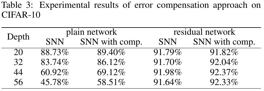
- shallow network. sampling error has no significant impact on performance
- deep network. actual max firing rate declines
- sampling error can be reduced by slightly enlarge the weights at each layer
- apply a compensation factor λ to each layer to reduce sampling errors by slightly enlarge the weights
- compensation factor λ is searched in a region of (1, τ_max). τ_max is the reciprocal firing max firing rate at last layer
3. Experiments
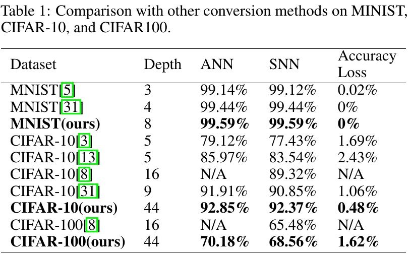
3.1. Comparison
3.2. Shortcut Normalization

3.3. ResNet vs CNN

3.4. Error Compensation